Note: Realized later on that what I was doing is procedurally generating tree graphics using L-systems. Didn’t know it at the time.

Symmetric Binary Trees

Reading this excellent book got me thinking on fractals in nature and how many natural structures could be modeled as neat self-referencing structures. I decided to try my hand at visually representing the most obvious choice for fractal structures in nature, which is trees, using python.

A tree can be thought of as a recursively generated object, with the main trunk splitting into a number of branches, and each branch further splitting in a similar way. To start simple, I write the following two functions to create a binary tree

def binary_tree(n,seed,changes):
    lines = []
    lines.append(seed)
    if n>1:
        new_seed1 = [(seed[0][0]+seed[1][0]*np.cos(seed[1][1]),seed[0][1]+seed[1][0]*np.sin(seed[1][1])),(seed[1][0]*changes[0],seed[1][1]+changes[1])]
        new_seed2 = [(seed[0][0]+seed[1][0]*np.cos(seed[1][1]),seed[0][1]+seed[1][0]*np.sin(seed[1][1])),(seed[1][0]*changes[0],seed[1][1]-changes[1])]
        lines.extend(binary_tree(n-1,new_seed1,changes))
        lines.extend(binary_tree(n-1,new_seed2,changes))
    return lines
	
	
def transform_tree_to_coord(tree_lines):
    tree_transf = [[(pt[0][0],pt[0][1]),(pt[0][0]+pt[1][0]*np.cos(pt[1][1]),pt[0][1]+pt[1][0]*np.sin(pt[1][1]))] for pt in tree_lines]
    return(tree_transf)
	

The function binary_tree is used to define a tree. Each tree is defined as a set of segments, with the segments defined recursively starting from the first, which I’ll call the trunk. Each segment is defined like a vector by $(x,y)$ coordinates for a point and $(l,\theta)$ for a length and direction. These are captured in the parameter seed which is [[x,y],[l,theta]]. For each segment, two new segments can be defined using the change parameter $(\alpha,\Delta\theta)$. The parameter n defines the depth to which this recursion is called, that is the depth of this tree. \([(x_{1},y_{1}),(l_{1},{\theta}_{1})] = [(x + l\cos(\theta),y + l\sin(\theta)),({\alpha}l,\theta+\Delta\theta)]\) \([(x_{2},y_{2}),(l_{2},{\theta}_{2})] = [(x + l\cos(\theta),y + l\sin(\theta)),({\alpha}l,\theta-\Delta\theta)]\)

This recursive multiplying, scaling and rotating leads to an exponentially growing tree fanning out from the trunk. The transform_tree_to_coord function merely transform the $[(x,y),(l,\theta)]$ coordinates into $[(x_1,y_1),(x_2,y_2)]$, which are the endpoints of the segment. This is useful merely for plotting purposes. Before plotting, widths for each segment are defined as proportional to their lengths.

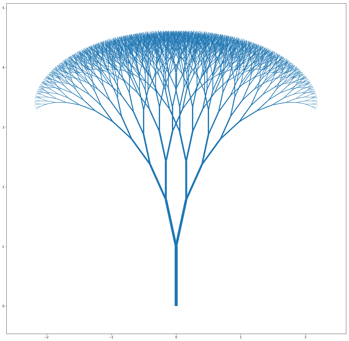
Plotting leads to some truly beautiful looking trees:

tree1_init = binary_tree(16, [(0,0),(1,np.pi/2)], [0.75,np.pi/8])
tree1 = transform_tree_to_coord(tree1_init)
widths1 = [10*pt[1][0] for pt in tree1_init]
lc = mc.LineCollection(tree1, linewidths=widths1)
fig, ax = pl.subplots(figsize=(20,20))
ax.add_collection(lc)
ax.autoscale()
ax.margins(0.1)

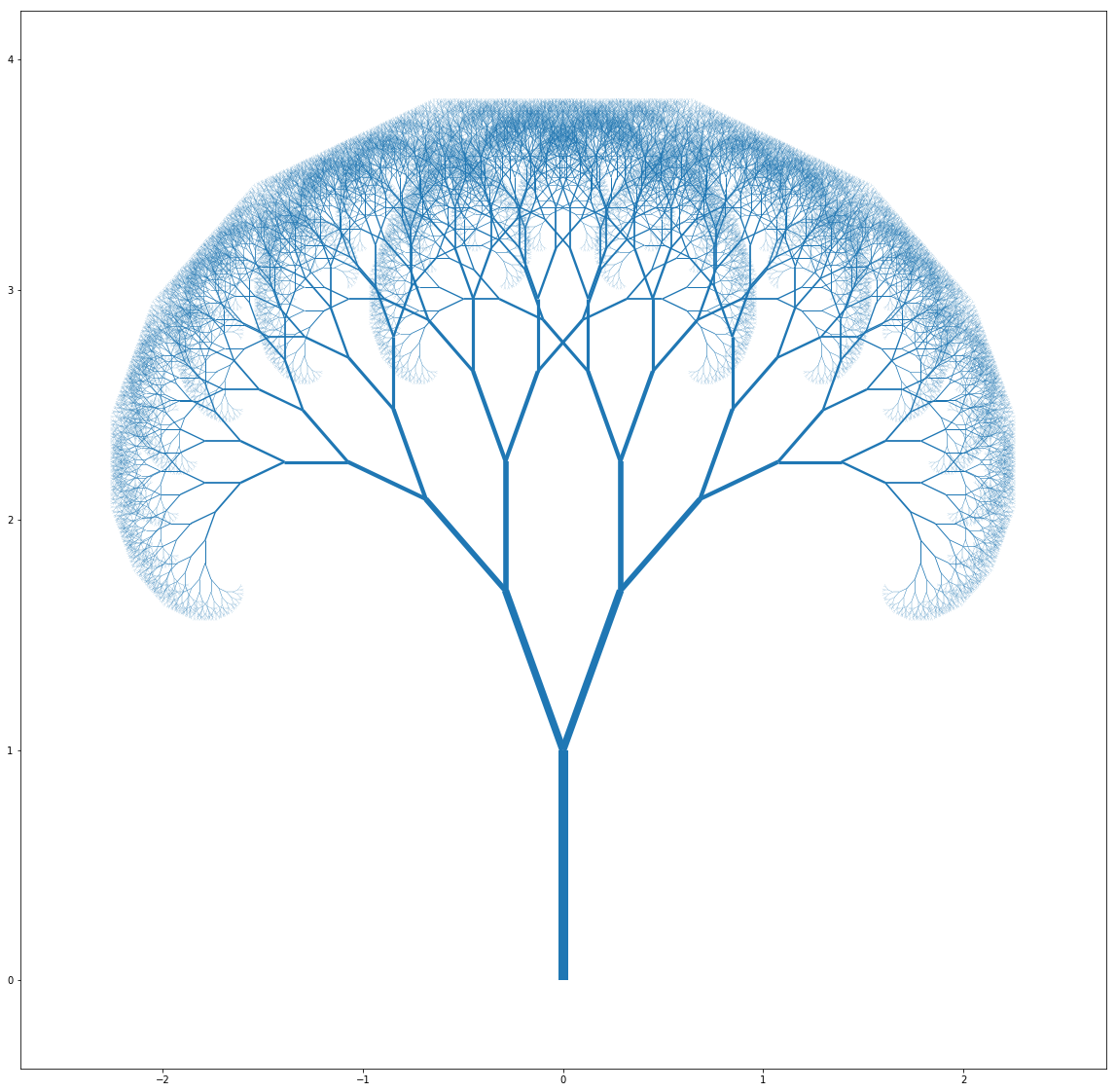
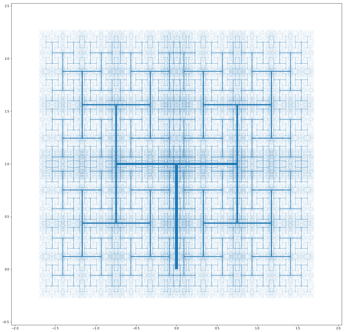
And pushing the parameters leads to some weird but interesting ones as well:

Random Trees

These binary trees still look very artificial and made up. How could we model infinite environmental stimuli and a tree’s reactions to them, which ultimately shape it’s structure? One way could be by defining a distribution and sampling from it at each recursive stage. This led me to define the following function:

def random_tree(n,seed,changes,branch_dist):
    lines = []
    lines.append(seed)
    if n>1:
        branches = np.random.choice(branch_dist[0],p=branch_dist[1])
        for b in range(branches):
            ang = np.random.uniform(low=-1,high=1)*changes[1]
            scale = np.random.uniform(low=0.8,high=1.2)*changes[0]
            new_seed = [(seed[0][0]+seed[1][0]*np.cos(seed[1][1]),seed[0][1]+seed[1][0]*np.sin(seed[1][1])),(seed[1][0]*scale,seed[1][1]+ang)]
            lines.extend(random_tree(n-1,new_seed,changes,branch_dist))
    return lines

The parameters n, seed, changes remain similar in meaning - except changes is now used to define distributions out of which angles and length scales are sampled from. A value for angular rotation is randomly chosen from a uniform distribution between $(-\Delta\theta,\Delta\theta)$, while a scaling factor is chosen from a uniform distribution between $(0.8l,1.2l)$. A new parameter branch_dist is defined which gives a list of probabilities for each number of branch splits. For example, $[(1,2,3,4),(0.6,0.3,0.07,0.03)]$ means that there is $60\%$ probability of only 1 branch at the next stage (no splitting), $30\%$ chance of splitting into 2 and so on. Number of branches at each recursive call are chosen according to these probabilities and scaling and rotation for each branch out of these chosen according to changes as mentioned before. A builder function is defined below which also takes another parameter width_mult. This is the proportionality factor for defining widths as proportional to lengths.

def build_tree_random(n,seed,changes,branch_dist,width_mult):
    tree_init = random_tree(n,seed,changes,branch_dist)
    tree = transform_tree_to_coord(tree_init)
    widths = [width_mult*(pt[1][0]**1.3) for pt in tree_init]
    return (tree,widths)

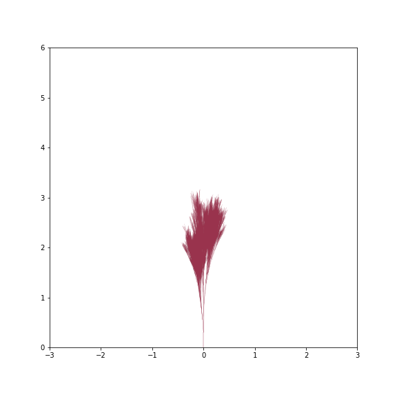
By just varying changes, branch_dist and width_mult we can get a surprising variety of trees - from grass like tufts to gnarly old trees Grass Tuft

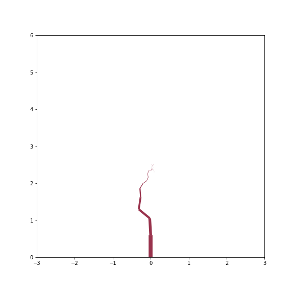Dried up sapling

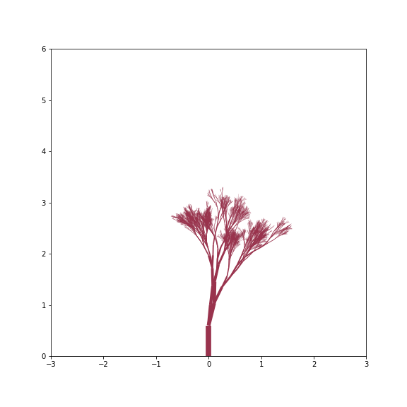Young Tree

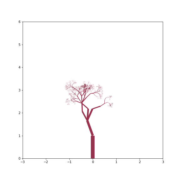Thin Tree

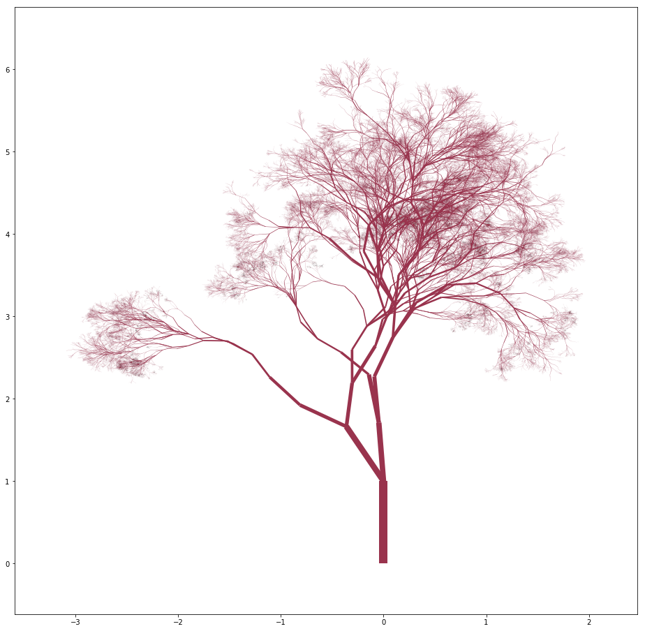Normal Tree

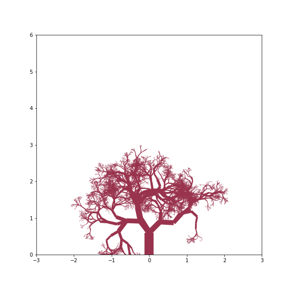Gnarly Tree

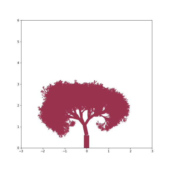Dense Tree

Forests

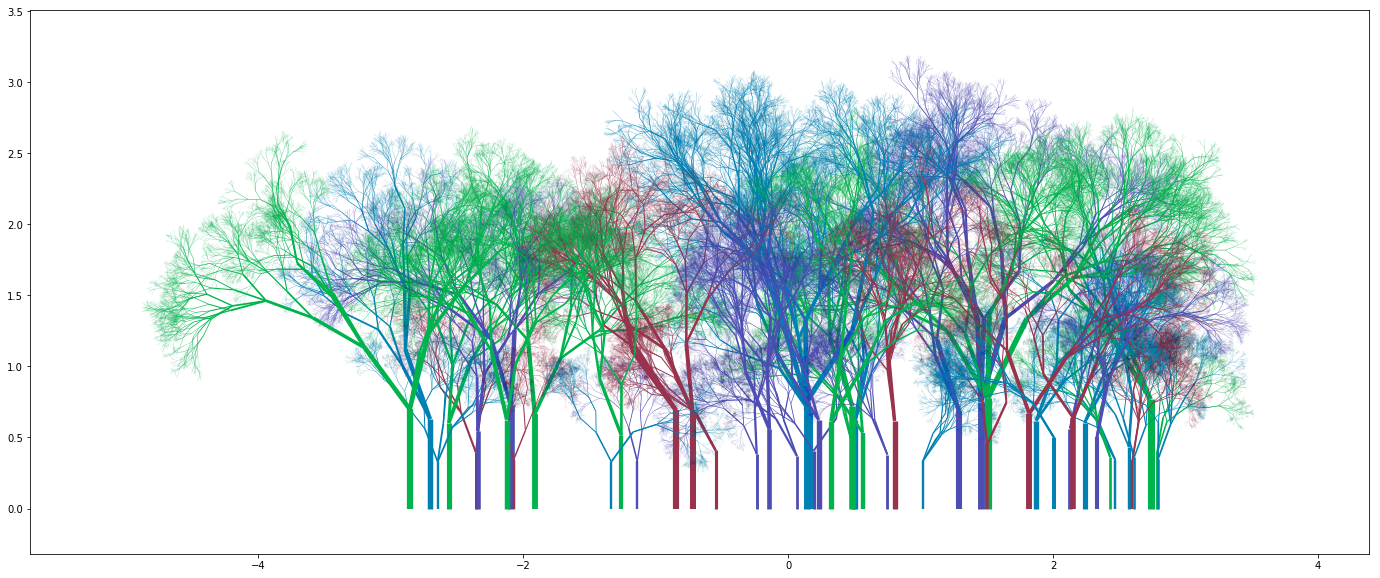
The fact that random sampling is involved in generation of a specific structure implies that similar looking but different trees can be generated with the same input parameters. Generating a grove of random trees - Random Forest - is the natural next step. For now I’ve kept the parameters (and thus style) of all trees in a forest constant, but this can be changed to have a distribution of styles to choose from as well.

def build_forest(num_trees,forest_width,color_map,n,seed,changes,branch_dist,width_mult):
    trees = []
    widths = []
    colors = []
    for t in range(num_trees):
        xshift_t = np.random.uniform(low=-1*forest_width,high=forest_width)
        lscale_t = np.random.uniform(low=0.1,high=1)
        
        seed_t = [(seed[0][0] + xshift_t,seed[0][1]),(seed[1][0]*lscale_t,seed[1][1])]
        tree_t,width_t = build_tree_random(n,seed_t,changes,branch_dist,width_mult)
        color_choice = color_map[np.random.choice(range(len(color_map)))]
        colors_t = [color_choice] * len(width_t)
        
        trees.extend(tree_t)
        widths.extend(width_t)
        colors.extend(colors_t)
    return (trees,widths,colors)

Some new parameters here - num_trees, forest_width and color_map. num_trees is simply the number of trees to be generated. forest_width defines the range of x values as $(-forest_width,forest_width)$ over which said trees will be placed randomly. color_map is a list of colors to be used for plotting trees. For each tree, a color is randomly chosen out of these. An example with sample parameters:

branch_dist1 = [[1,2,3,4],[0.4,0.4,0.15,0.05]]
color_map = [(0,0.7,0.3,1),(0.3,0.3,0.7,1),(0,0.5,0.7,1),(0.6,0.2,0.3,1)]
w=5
trees,widths,colors = build_forest(85,w,color_map,16, [(0,0),(0.8,np.pi/2)], [0.75,np.pi/5],branch_dist1,15)

lc = mc.LineCollection(trees, colors=colors,linewidths=widths)
fig, ax = pl.subplots(figsize=(8*w,12))
ax.add_collection(lc)
ax.autoscale()

You can get some really nice looking groves:

What next?

There can be several ways this concept can be further explored.

• Trees: Bias can be introduced to branch rotation angle sampling leading to more inward or outward growing trees. Similar biases in sampling other aspects can also be implemented.
• Forests: Forests can have multiple types of trees, some more numerous than others. This can be achieved using a probability distribution of styles from which to choose from.
• Forests: Height of seed can be generated based on size, to add the illusion of depth. All trees start from x-axis right now. If some trees were smaller and started slightly above at some positive y value, it would seem as if they’re farther away from the viewer.
• Other structures: Fractal nature can be seen in a lot of natural structures such as seacoasts, mountains and so on. Some sort of implementation similar to this can be generated for those as well.